Build a Network Layer Visualization with Checkmk

In an increasingly distributed world, having a visual way to see how your networks are connected and if there are hosts with problems is an invaluable help to administrators. It makes it simpler to understand how an infrastructure is interconnected and of what it is made of.

The network visualization is a graphical backend built into Checkmk to show connections between objects. These objects can be hosts and services of hosts from your Checkmk instance or any objects that are not part of the Checkmk instance, e.g. IP addresses, IP networks, clouds or whatever you want. Theoretically-speaking objects can be anything, like a collection of toy building blocks or the local railway network, but we will focus exclusively on IT network infrastructures.

The purpose of visualizing these connections is to give you a better understanding of how the components of your IT infrastructure are connected, which can help you find misconfigurations between devices (e.g. connections with different interface speeds) or interrupted links.

The network topology in Checkmk collects its info via two common protocols for this task: CDP and LLDP. The former, Cisco Discovery Protocol, is present on mainly Cisco devices but has been implemented by other vendors as well. It is probable you will have it available in your infrastructure. The second protocol, Link Layer Discovery Protocol, is vendor-neutral. Both operate on the OSI layer 2 level, so we are talking of info below the IP addresses like ARP tables and MAC addresses.

Moreover, IP-level topology is also supported. That is OSI layer 3, and operates on IP addresses. This will cover your Windows, Linux, and SNMP network devices, including them in the topology.

Regardless of choosing CDP or LLDP or going with IP, it is recommended to choose what best suits your needs or environment.

Let’s see how the network visualization in Checkmk looks like with a small example:

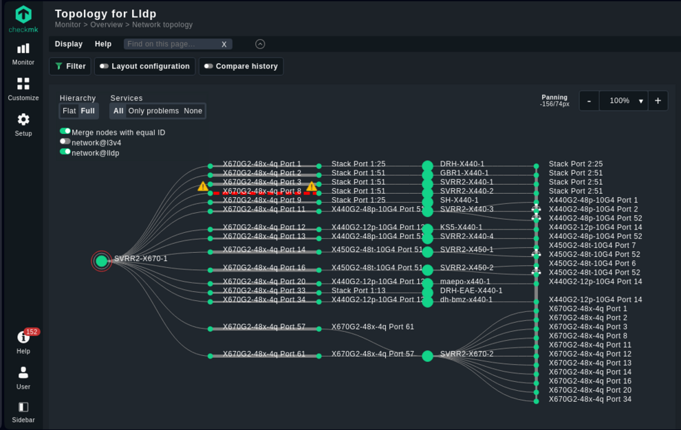
The topology above was created from the LLDP information of monitored switches, present in Checkmk’s HW/SW inventory. Probably it is clearer to see how the root nodes and switches are connected, and what services they are running in the next animated gif:

We can see here the root nodes on the left, the connected switches on the right, and the various interfaces that connect them in between. Information about the node/service is given in a hover tooltip over the icons.

Further information can be gleaned from the lines connecting the devices and services:

The thickness can be used to show the bandwidth, the color to show issues (like red for a slow connection).

Filters are available on the right side of the screen, as usual in the Checkmk interface:

In the animated GIF above are demonstrated the display options to show or hide labels and whole interfaces. These filters are in real-time, no need to apply them.

This is what it looks like and what it can do. Let's see how to set it up.

The setup of the network topology visualization is straightforward now. The required mainline network topology inventory plug-ins are natively built into Checkmk since 2.5.0. This means you immediately have access to:

• Layer 2 topology plug-ins: CDP and LLDP inventory plug-ins.
• Layer 3 topology plug-ins: IP inventory plugins for SNMP, Windows, and Linux.
• Additional plug-ins: Interface name inventory plug-in.

Previously, populating the Checkmk HW/SW inventory required administrators to manually download and install multiple external plug-ins (CDP, LLDP, IPv4, and INV_IFNAME). This is not needed anymore in 2.5. 

Be aware that if you came from a previous Checkmk and NVDCT setup and rely on custom rules or scripts that reference the old nvdct/ host labels, you must update them to the new cmk/ labels to maintain compatibility. Additionally, inventory tables have been renamed to en-us and table headers now follow sentence case formatting, though this will not affect your workflows or integrations.

For this setup, Checkmk already includes all required packages out of the box. The only exception is the Network Visualization Data Creation Tool (NVDCT) plug-in, which you still need to install manually. You can install it as usual through Checkmk's GUI via Setup > Extension Packages > Upload package. Users of Checkmk Community will have to install it via CLI with:​​​​​​​

The NVDCT tool relies on certain host labels discovered via the built-in plugins.

Important: Checkmk 2.5+ uses the cmk/ prefix for all topology-related host labels. All references that previously used the nvdct/ prefix have been replaced by their cmk/ equivalents.

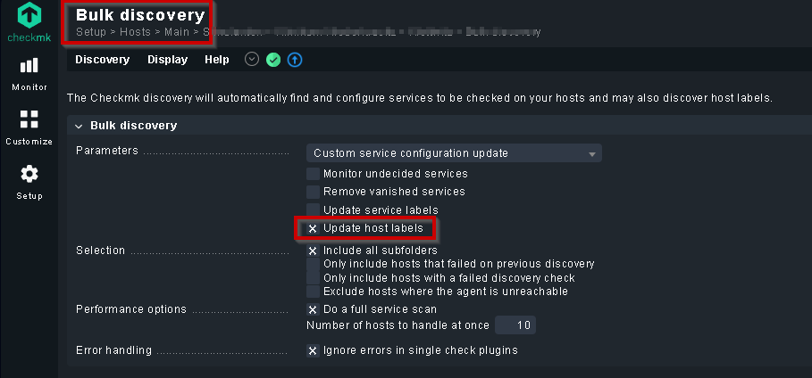
These labels can speed up the creation of the data file and are mandatory for Layer 3 IP topologies, as neighbor information is not available natively like it is with CDP/LLDP. Please make sure to update the host labels, for example using the bulk discovery:

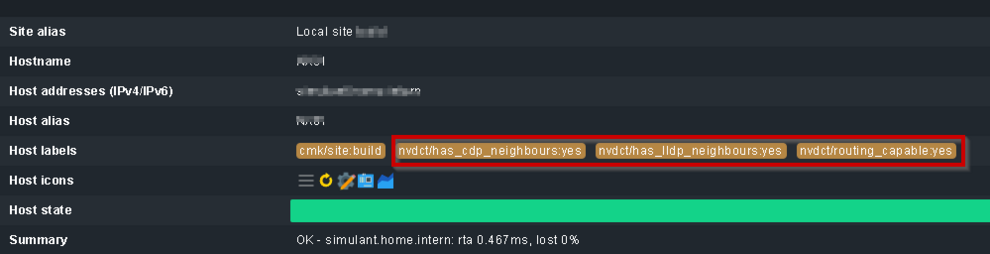
When the host label discovery is finished, you can review the discovered host labels:

HW/SW inventory must be enabled for all the network devices that you want to include in the topology via the rule “Do hardware/software inventory”. The advised check interval is 24 hours. The HW/SW inventory must be run before NVDCT to allow the plug-in to collect the reported data and build the network topology from it.

After the HW/SW inventory is run successfully you can check the results.

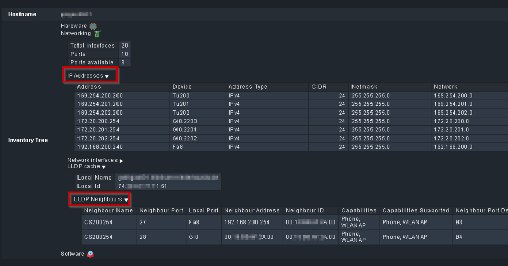
If your device has CDP neighbors, you should also see a table for CDP like the table for LLDP.

Once the NVDCT package is installed, the rules are set, the HW/SW inventory has run, and the cmk/ labels are discovered, it's time to start with the topology creation.

First, look at the configuration file at ~/local/bin/nvdct/conf/nvdct.toml. Create a personal copy before modifying it so updates don't overwrite your settings. For the CDP/LLDP layer, you should add your seed devices (from which NVDCT starts creating the topology) in the SEED_DEVICES section of the TOML file, as shown below:

# list of seed devices
SEED_DEVICES = [
    "DEVICE01",
    "DEVICE02",
    "DEVICE03",
]

In the [SETTINGS] section, enable the layers you want to create (e.g., LLDP, CDP, L3v4):

# settings equivalent to CLI options
[SETTINGS]
# layers = ["LLDP", "CDP", "STATIC", "CUSTOM", "L3v4"]
layers = ["LLDP", "L3v4"]

Once satisfied with the content of the configuration file, create your network topology by running:

~$ ~/local/bin/nvdct/conf/nvdct.py -c ~/local/bin/nvdct/conf/my_nvdct.toml

Which will output something similar to:

Network Visualisation Data Creation Tool (NVDCT)
by thl-cmk[at]outlook[dot]com, version 0.8.7-20240430
see https://thl-cmk.hopto.org/gitlab/checkmk/vendor-independent/nvdct

Start time....: 2024-04-30T14:17:02.04
Devices added.: 16, source lldp
Devices added.: 59, source L3v4
Time taken....: 3.225333135/s
End time......: 2024-04-30T14:17:05.04
~$

The created topology data will be found under ~/var/check_mk/topology/data/

A symbolic link to the default topology will be also present:

~$ ls -ls ~/var/check_mk/topology/data
4 drwx------ 2 build build 4096 Apr 30 14:17 2024-04-30T14:17:05.04/
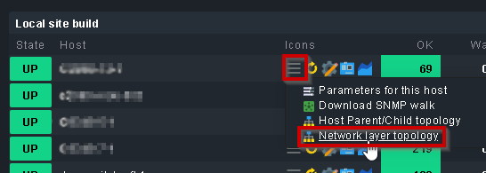
0 lrwxrwxrwx 1 build build   57 Apr 30 14:25 default -> /omd/sites/build/var/topology_data/2024-04-30T14:17:05.04/

The generated topology will be now accessible in the host menu in Checkmk, selecting the “Network layer topology” option, as shown in the screenshot below. Start with one of your seed devices to explore the Network topology.

No matter how you create the network topology, by hand or with the NVDCT package, there are a lot of customization possibilities in Checkmk. The default info shown is the hosts relationship with the interfaces. It is also visible the current status of hosts and services, with a link to the appropriate view. If desired, services can be hidden to reduce visual clutter, or only shown services with problems, thanks to the switch in the top left of the visualization.

It is possible to visually compare two data sets from different points in time. This is the “compare history” in the options, as seen below:

First you select a reference time, usually the current time. and then you select the comparison time. The topology then determines any differences in the connections between the two timestamps. namely connections that are missing in the reference and connections that only exist in the reference.

Visualization styles are available. Currently you can switch between two ready-made layouts for displaying the data: full and flat.

The full layout gives you a better view of the connections, as these are visualized in a tree structure. The flat layout is more compact, easier to read at a glance but keeping the full connections data when hovering over the nodes and connections.

Alternatively, you can use the ‘layout configuration’ feature to generate a completely free layout, which is automatically loaded when this view is called up with the exact same filter settings.

On top of the visualization there are a few interesting features. You can filter the network topology, and configure its layout. Filters are customizable, you can add yours. By default the most common ones are present, such as:

• Topology max nodes
• Topology mesh depth
• Hostname (regex)
• Hostalias (regex)
• Several host groups
• Host Contact Group
• Host states
• Host labels
• Host tags
• Site

A word more is needed for the first two filters. Topology max nodes specifies how many nodes should be shown and if the selected limit is reached, a warning is displayed in the title.

Topology max depth is useful to limit the travel to build the topology to a number of hops from the start node or nodes.

It is also possible to compare the differences between two timestamps, to visually check what changed between two times. With NVDCT you can style the topology with different icons, a custom color for the lines, thicker connections and more.

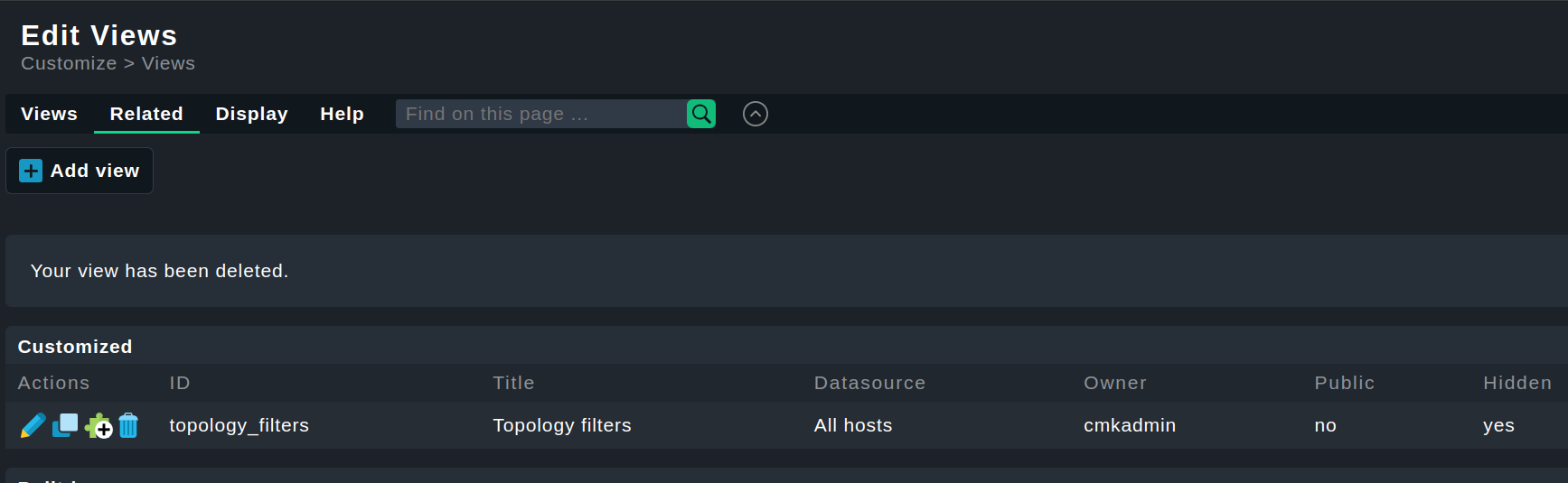
There is also a built-in filter to customize the default visualization parameters. It is called topology_filters. Clone it and adjust its parameters to your preference.

The topology uses one data file for each data type for a given timestamp. It can grow quite numerous but not very large, as they are all simple TOML files. There are two main components of the data:

• The objects, representing the nodes in the visualization
• The connections, representing the relationships between nodes

An example of a data file is shown below:

{
    "version": 1,       # data format version
    "name": "CDP data", # some name to display somewhere
    "objects": {        # A dictionary containing the object ID key and the object as value
        # A generic node with the ID NodeA and the display name 'NodeA'
        # It is a simple node with no relationship to the monitoring core
        'NodeA': {'metadata': {}, 'name': 'NodeA'},

        # A node with the ID HostA_ID, which is linked to a host 'HostA' in the core.
        # In the visualization the node is named 'HostA Name'
        'HostA_ID': {'link': {'core': 'HostA'}, 'metadata': {}, 'name': 'HostA Name'},

        # A node with the ID HostA_ServiceX, which is linked to a service
        # 'HostA'/'ServiceX' in the core. In the visualization the node is named 'Service X'
        'HostA_ServiceX': {'link': {'core': ['HostA', 'ServiceX']}, 'metadata': {}, 'name': 'Service X'},

        # The metadata field is used to add additional information.
        # A generic node with the ID NodeWithImages and the display name 'ImageNode'
        # This generates a node which is shown in the screenshot above
        'NodeWithImages': {'metadata': {
                             'images': {"icon": "icon_checkmark", "emblem": "emblem_warning"}
                           },
                           'name': 'ImageNode'},
    },
    # The objects are always identified by their ID
    # A connection always connects two objects and has tree values [SOURCE_ID, TARGET_ID, metadata]
    "connections": [
        # A simple connection between NodeA and HostA_ID
        [["NodeA"], ["HostA_ID"], {}],
        # Another simple connection between NodeA and HostA_ServiceX
        [["NodeA"], ["HostA_ServiceX"], {}],
        # A connection between HostA_ServiceX and NodeWithImages.
        # The line_config field specifies the custom styling
        [["HostA_ServiceX"], ["NodeWithImages"], {"line_config": {"thickness": 5, "color": "green"}}],
    ]
}

Important to note are the indices "images" and "line_config". The index “images” has two keys:

• “icon”: an icon to display at the top left of the node, which overrules pre-configured icons in the core
• “emblem”: an image to replace the blue question mark on nodes that are not linked to the core

The index “line_config” has two keys as well:

• “thickness”: the desired thickness of the connection
• “color”: the color of the connection. Color names and HEX color codes are both accepted here